Overview
Our model achieves outstanding performance in predicting Sea Surface Temperature patterns, capturing both short-term fluctuations and long-term trends with remarkable accuracy.
SINDy-SHRED accurately predicts complex motion patterns in video sequences, maintaining physical consistency even over extended prediction horizons.
SINDy-SHRED demonstrates exceptional performance in capturing the complex vortex shedding patterns and flow dynamics around a cylinder, showcasing its ability to model fluid dynamics phenomena.
Our model successfully captures the intricate structures and energy cascade in isotropic turbulent flow, demonstrating its capability to handle complex turbulent dynamics.
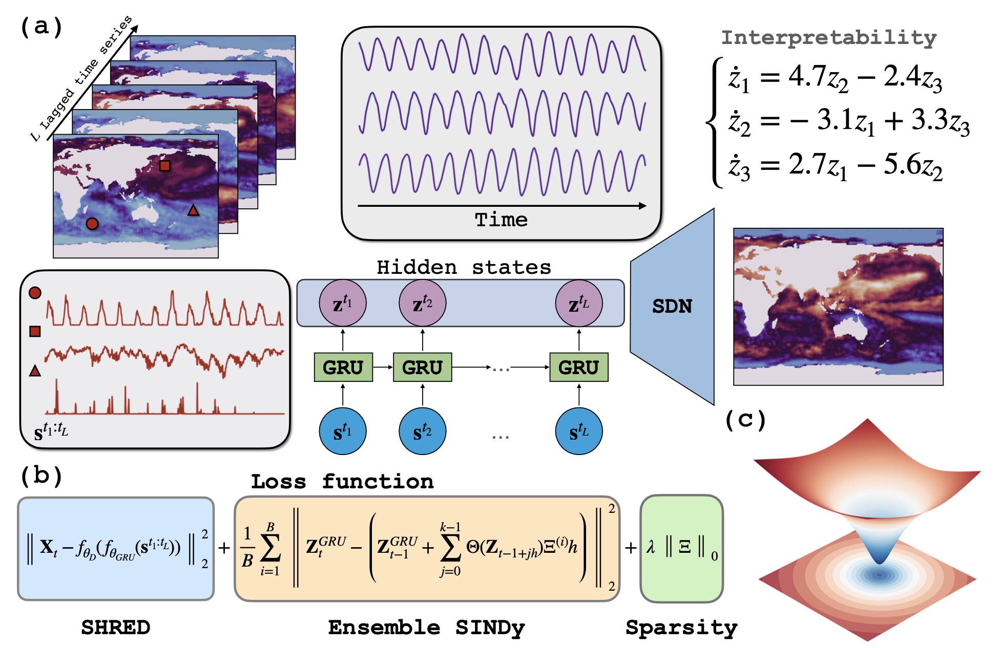
The loss landscape visualization reveals the globally convex nature of our optimization problem, explaining the model's robust convergence and stability during training.
| Models | Params | Training time | T=[0,100] | T=[100,200] | T=[200,275] | Total |
|---|---|---|---|---|---|---|
| ResNet | 2.7M | 24 mins | 2.08×10⁻² | 1.88×10⁻² | 2.05×10⁻² | 2.00×10⁻² |
| SimVP | 460K | 30 mins | 2.29×10⁻² | 2.47×10⁻² | 2.83×10⁻² | 2.53×10⁻² |
| PredRNN | 444K | 178 mins | 1.02×10⁻² | 1.79×10⁻² | 1.69×10⁻² | 1.48×10⁻² |
| ConvLSTM | 260K | 100 mins | 9.24×10⁻³ | 1.86×10⁻² | 1.99×10⁻² | 1.55×10⁻² |
| SINDy-SHRED* | 44K | 17 mins | 1.70×10⁻² | 9.36×10⁻³ | 5.31×10⁻³ | 1.05×10⁻² |
We strongly encourage you to explore SINDy-SHRED by directly running our Colab notebook:
Open in ColabVideo tutorial to learn about SINDy-SHRED
import sindy_shred
validation_errors = sindy_shred.fit(
    shred,
    train_dataset,
    valid_dataset,
    batch_size=128,
    num_epochs=600,
    lr=1e-3,
    verbose=True,
    threshold=0.25,
    patience=5,
    sindy_regularization=10.0,
    optimizer="AdamW",
    thres_epoch=100
)

print(f"Final validation error: {validation_errors[-1]:.6f}")
# Import required libraries
latent_dim = 3
poly_order = 3
include_sine = False
library_dim = sindy.library_size(latent_dim, poly_order, include_sine, True)

# Initialize SINDy-SHRED model
shred = sindy_shred.SINDy_SHRED(
    num_sensors=num_sensors,
    m=m,  # Full state dimension
    hidden_size=latent_dim,
    hidden_layers=2,
    l1=350,
    l2=400,
    dropout=0.1,
    library_dim=library_dim,
    poly_order=poly_order,
    include_sine=include_sine,
    dt=1/52.0*0.1,
    layer_norm=False
).to(device)
# Import required libraries
import numpy as np
from processdata import load_data, TimeSeriesDataset
import torch
from sklearn.preprocessing import MinMaxScaler
import os

# Set up device and parameters
os.environ["CUDA_VISIBLE_DEVICES"] = "0"
device = 'cuda' if torch.cuda.is_available() else 'cpu'
num_sensors = 250
lags = 52

# Load and preprocess data
load_X = load_data('SST')
n, m = load_X.shape
sensor_locations = np.random.choice(m, size=num_sensors, replace=False)

# Split data into train/valid/test
train_indices = np.arange(0, 1000)
mask = np.ones(n - lags)
mask[train_indices] = 0
valid_test_indices = np.arange(0, n - lags)[np.where(mask!=0)[0]]
valid_indices = valid_test_indices[:30]
test_indices = valid_test_indices[30:]

# Scale the data
sc = MinMaxScaler()
sc = sc.fit(load_X[train_indices])
transformed_X = sc.transform(load_X)

# Generate input sequences
all_data_in = np.zeros((n - lags, lags, num_sensors))
for i in range(len(all_data_in)):
    all_data_in[i] = transformed_X[i:i+lags, sensor_locations]

# Create datasets
train_data_in = torch.tensor(all_data_in[train_indices], dtype=torch.float32).to(device)
valid_data_in = torch.tensor(all_data_in[valid_indices], dtype=torch.float32).to(device)
test_data_in = torch.tensor(all_data_in[test_indices], dtype=torch.float32).to(device)

train_data_out = torch.tensor(transformed_X[train_indices + lags - 1], dtype=torch.float32).to(device)
valid_data_out = torch.tensor(transformed_X[valid_indices + lags - 1], dtype=torch.float32).to(device)
test_data_out = torch.tensor(transformed_X[test_indices + lags - 1], dtype=torch.float32).to(device)

train_dataset = TimeSeriesDataset(train_data_in, train_data_out)
valid_dataset = TimeSeriesDataset(valid_data_in, valid_data_out)
test_dataset = TimeSeriesDataset(test_data_in, test_data_out)
Note: For a step-by-step guide, please check out our Google Colab notebook.
SINDy-SHRED offers several key advantages over traditional methods:
For D-dimensional fields, SINDy-SHRED requires only D+1 sensors for disambiguation of the spatiotemporal field, similar to localization in cellular networks. However, to get a stable latent space, we recommend using around 0.5% of the total number of sensors.
If you find SINDy-SHRED useful in your research, please cite:
@misc{gao2025sparse,
      title={Sparse identification of nonlinear dynamics and Koopman operators with Shallow Recurrent Decoder Networks},
      author={Mars Liyao Gao and Jan P. Williams and J. Nathan Kutz},
      year={2025},
      eprint={2501.13329},
      archivePrefix={arXiv},
      primaryClass={cs.LG},
      url={https://arxiv.org/abs/2501.13329},
}